Rでエッジワース・ボックスを描こう

Edgeworth Box

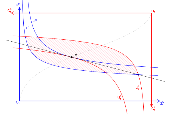
以前に描いたコードを整理しなおしたと言うか、手計算で微分して均衡や契約曲線を求めていたのでどちらかと言うと作り直したものですが、applyやwhichやexpressionなどに慣れるのに良さそうだったので。数値解析で均衡点を求めているので、初期財の配分を変えたり、効用関数を他の凸で連続なモノ（e.g. CES型）に変えても、そこの部分だけの変更でプロットできるはずです。

# 連立方程式を解くのでnleqslvをロード、インストールしていなければインストールしてもらう
loadLib <- function(...){
    for(lname in unlist(list(...))){
        if(!any(suppressWarnings(library(quietly=TRUE, verbose=FALSE)$results[,"Package"] == lname))){
            stop(sprintf("Do install.packages(\"%s\") before runnning this script.", lname))
        }
        library(lname, character.only = TRUE)
    }
}

loadLib("nleqslv")

# 財の配分を表す行列
initial_goods <- matrix(c(0.9, 0.1, 0.3, 0.7), 2, 2,
    dimnames = list(c("person 1", "person 2"), c("g/s A", "g/s B")))

# トランスログ型効用関数の雛形を定義
U_pt <- function(b, gs_a, gs_b){
    # b[3]～b[5]≠0だと局所的に凸なだけなので、安易に財の総量を増やしたり、下手にパラメーターをいじると、計算がデタラメに。
    if(gs_a <=0 || gs_b<=0) return(-Inf)
    as.numeric(b[1]*log(gs_a) + b[2]*log(gs_b) + b[3]*log(gs_a)^2 + b[4]*log(gs_b)^2 + b[5]*log(gs_a)*log(gs_b))
}

# Person 1と2の効用関数を定義
U_1 <- function(gs_a, gs_b) U_pt(c(0.4, 0.6, 0, -0.5, 0), gs_a, gs_b)
U_2 <- function(gs_a, gs_b) U_pt(c(0.5, 0.5, 0, -0.4, 0), gs_a, gs_b)

# 各財/サービスの合計を求めておく
sum_of_goods <- apply(initial_goods, 2, sum)

# グラディエントを数値解析
dU <- function(U, gs_a, gs_b, h=1e-4){
	r <- c(U(gs_a + h, gs_b) - U(gs_a - h, gs_b),
    U(gs_a, gs_b + h) - U(gs_a, gs_b - h)) / (2*h)
    names(r) <- c("d(g/s A)", "d(g/s B)")
    r
}

getPrice <- function(goods){
    # 限界効用を計算
    dU1 <- dU(U_1, goods["person 1", "g/s A"], goods["person 1", "g/s B"])
    dU2 <- dU(U_2, goods["person 2", "g/s A"], goods["person 2", "g/s B"])

    # 価格と言うか交換レート（限界代替率）を計算
    r <- c(dU1["d(g/s A)"]/dU1["d(g/s B)"], dU2["d(g/s A)"]/dU2["d(g/s B)"])
    names(r) <- c("person 1", "person 2")
    r
}

getDistribution <- function(initial_goods, exchange){
    # 財配分を更新
    # initial_goods: 初期配分
    # exchange: 交換量
    goods <- initial_goods
    goods["person 1", ] <- initial_goods["person 1", ] - exchange
    goods["person 2", ] <- initial_goods["person 2", ] + exchange
    goods
}

getEquilibrium <- function(initial_goods){
    # 均衡を計算

    r_nleqslv <- nleqslv(c(0.0, -0.0), function(exchange){
        goods <- getDistribution(initial_goods, exchange)
        p <- getPrice(goods)
        # Person 1とPerson 2の限界代替率が一致し、Person 1の支出と収入が一致する点が均衡
        # p*(x0 - x) + (y0 - y) = 0
        c(p["person 1"] - p["person 2"], exchange[1]*p["person 1"] + exchange[2])
    }) 

    exchange <- r_nleqslv$x
    goods <- getDistribution(initial_goods, exchange)
    price <- getPrice(goods)

    # 分離超平面（式の形にしておく）
    shpe <- substitute(B0 - a*(A - A0), list(B0=goods[1, 2], a=price[1], A0=goods[1, 1]))

    list(price=price, exchange=exchange, goods=goods, shp=function(A){ eval(shpe) })
}

# 均衡の計算
equilibrium <- getEquilibrium(initial_goods)

# 無差別曲線の描画
drawIDC <- function(goods, lwd=c(1.5, 1.5), col=c("blue", "red", "pink"), names=NULL, IsCore=FALSE, density=10){
    UL_1 <- U_1(goods["person 1", "g/s A"], goods["person 1", "g/s B"])
    UL_2 <- U_2(goods["person 2", "g/s A"], goods["person 2", "g/s B"])

    demand_B <- function(UL, U, A){
        B <- numeric(length(A))
        for(i in 1:length(A)){
            r_nlm <- nlm(function(b){
                    if(b <= 0){
                        return(1e+6)
                    }
                    (UL - U(A[i], b))^2
            }, 1)
            B[i] <- with(r_nlm, ifelse(code<=3, estimate[1], NA))
        }
        B
    }

    # 財Aの量が横軸になる，0は効用関数の定義域から外れるので調整している
    # 無差別曲線を2つ、片方ひっくり返して重ねている図のため、線が枠をはみ出る方がよいので、上限はあえてずらしてる
    scale <- 1.05
    A <- seq(1e-6, sum_of_goods["g/s A"]*scale, length.out=101)

    IC_1 <- matrix(c(A, demand_B(UL_1, U_1, A)),
        length(A), 2)
    colnames(IC_1) <- c("g/s A", "g/s B")

    # Person 2の無差別曲線は180度回転してプロットするため、経済全体の財の量からPerson 2の財の量を引いて、対応するPerson 1の財の量を求めてプロットしている
    IC_2 <- matrix(c(sum_of_goods["g/s A"] - A,
        sum_of_goods["g/s B"] - demand_B(UL_2, U_2, A)),
        length(A), 2)
    colnames(IC_2) <- c("g/s A", "g/s B")

    lines(IC_1[,"g/s B"] ~ IC_1[,"g/s A"], lwd=lwd[1], col=col[1])
    lines(IC_2[,"g/s B"] ~ IC_2[,"g/s A"], lwd=lwd[2], col=col[2])

    if(!is.null(names)){
        # 描画域の大きさから、表示位置の調整量を決める
        xadj <- (par()$usr[2] - par()$usr[1])/75

        # 枠内で最大のB財の量を求める
        b <- max(IC_1[ , "g/s B"][IC_1[ , "g/s B"] < sum_of_goods["g/s B"]], na.rm = TRUE)
        # 最大のB財に対応する行を求める
        i <- which(IC_1[ , "g/s B"]==b, arr.ind=TRUE)
        text(IC_1[i, "g/s A"] + xadj, b, names[1], col=col[1], adj=c(0, 1))

        # 枠内で最小のB財の量を求める
        b <- min(IC_2[ , "g/s B"][IC_2[ , "g/s B"] > 0], na.rm = TRUE)
        # 最小のB財に対応する行を求める
        i <- which(IC_2[ , "g/s B"]==b, arr.ind=TRUE)
        text(IC_2[i, "g/s A"] - xadj, b, names[2], col=col[2], adj=c(1, 0))
    }

    # 純粋交換経済のコア
    # Person 2の無差別曲線（の180度回転）のB財の量よりも、Person 1のB財の量が同じか少ない領域を求める
    if(IsCore){
        # 横軸のIC_1の財Aの量とIC_2の財Aの量の対応がずれているので、線形近似関数をつくる
        af_1 <- approxfun(IC_1[ , "g/s A"], IC_1[ , "g/s B"])
        af_2 <- approxfun(IC_2[ , "g/s A"], IC_2[ , "g/s B"])
        # 横軸を細かく取り直す
        A <- seq(1e-6, sum_of_goods["g/s A"]-1e-6, length.out=100)
        A <- A[af_1(A) <= af_2(A)]
        # コアの周回経路を求める
        x <- c(A, rev(A)) # 行きと帰りは向きが逆
        y <- c(af_1(A), af_2(rev(A))) # 行きはPerson 1の無差別曲線に沿って、帰りはPerson 2の〃
        # 面を書く関数で色を塗る
        polygon(x, y, density=density, col=col[3], border=NA)
    }

}

# 背景を白に、余白を小さくして、フォントサイズを大きくした設定にする
par(bg="white", mar=c(0, 0, 0, 0), cex=1)

# 低水準グラフィックス関数で描いて行く
plot.new()
margin <- 0.1
xlim <- c(-margin, (1 + margin))*sum_of_goods["g/s A"]
ylim <- c(-margin, (1 + margin))*sum_of_goods["g/s B"]
plot.window(xlim=xlim, ylim=ylim)

col <- c("blue", "red")

# 枠と言うか矢印を書く
with(list(l=0.125, lwd=2), {
    xlim <- c(-l/2, (1.0 + l/2))*sum_of_goods["g/s A"]
    ylim <- c(-l/2, (1.0 + l/2))*sum_of_goods["g/s B"]

    arrows(0.0, 0.0, xlim[2], 0, col=col[1], lwd=lwd, length=l)
    arrows(0.0, 0.0, 0, ylim[2], col=col[1], lwd=lwd, length=l)

    arrows(sum_of_goods["g/s A"], sum_of_goods["g/s B"], sum_of_goods["g/s A"], ylim[1], col=col[2], lwd=lwd, length=l)
    arrows(sum_of_goods["g/s A"], sum_of_goods["g/s B"], xlim[1], sum_of_goods["g/s B"], col=col[2], lwd=lwd, length=l)

    text(0, 0, expression(O[1]), col=col[1], adj=c(1, 1))
    text(xlim[2], 0, expression(G[1]^A), col=col[1], adj=c(0, 1))
    text(0, ylim[2], expression(G[1]^B), col=col[1], adj=c(1, 0))

    text(sum_of_goods["g/s A"], sum_of_goods["g/s B"], expression(O[2]), col=col[2], adj=c(0, 0))
    text(xlim[1], sum_of_goods["g/s B"], expression(G[2]^A), col=col[2], adj=c(1, 0))
    text(sum_of_goods["g/s A"], ylim[1], expression(G[2]^B), col=col[2], adj=c(0, 1))
})

# 契約曲線の計算と描画

# 初期時点の組み合わせを格子状に大量に作って計算する
grid <- expand.grid(
    # 0は効用関数の定義域から外れるので調整している
    "g/s A"=seq(1e-2, 1 - 1e-2, length.out=11) * sum_of_goods["g/s A"],
    "g/s B"=seq(1e-2, 1 - 1e-2, length.out=11) * sum_of_goods["g/s B"])

# apply関数で行列の列ごとに操作する
r_apply <- apply(grid, 1, function(goodsOfPrsn1){
    goods <- matrix(c(goodsOfPrsn1, sum_of_goods - goodsOfPrsn1),
        2, 2, dimnames=dimnames(initial_goods), byrow=TRUE)
    equilibrium <- getEquilibrium(goods)
    with(equilibrium, c(goods["person 1", "g/s A"], goods["person 1", "g/s B"]))
})

# 表示する均衡点も契約曲線の点の集合に入れておく
r_apply <- cbind(r_apply, with(equilibrium, c(goods["person 1", "g/s A"], goods["person 1", "g/s B"])))

# 行に名前をつけておく
rownames(r_apply) <- c("g/s A", "g/s B")

# A財の大小で並び替えておく
r_apply <- r_apply[, order(r_apply["g/s A", ])]

# 直線でつないで契約曲線の近似とする
lines(r_apply["g/s A", ], r_apply["g/s B", ], lty=3, col="darkgray")

# 初期点を通る無差別曲線を描画
drawIDC(initial_goods, names=c(expression(U[1]^I), expression(U[2]^I)), IsCore=TRUE)

with(equilibrium, {
    # 均衡を通る無差別曲線を描画
    drawIDC(goods, col=col, names=c(expression(U[1]^E), expression(U[2]^E)))

    xadj <- (par()$usr[2] - par()$usr[1])/50 # 文字表示の位置調整
    pch <- 21 # 点の形状（21:丸, 22:四角, 23:菱形, 24:三角，25:逆三角, etc...）

    # 初期配分を描画
    points(initial_goods["person 1", "g/s A"], initial_goods["person 1", "g/s B"], pch=pch, col="blue", bg="blue")
    text(initial_goods["person 1", "g/s A"] + xadj, initial_goods["person 1", "g/s B"], expression(I), adj=c(0, 0))

    # 競争均衡点を描画
    points(goods["person 1", "g/s A"], goods["person 1", "g/s B"], pch=pch, col="black", bg="black")
    text(goods["person 1", "g/s A"] + xadj, goods["person 1", "g/s B"], expression(E), adj=c(0, 0))

    # 分離超平面を描画
    A <- seq(xlim[1], xlim[2], length.out=2)
    lines(A, shp(A))
})

# 画像ファイルの保存先ディレクトリをつくる
img_path <- "img"
if(!dir.exists(img_path)){
    dir.create(img_path)
}

# プロットを画像ファイルにコピーして保存
dev.copy(png, file=sprintf("%s/edgeworth_box.png", img_path), width=600, height=400, type="cairo"); dev.off() # , type="cairo"でアンチエイリアス

Rのリスト処理のざっとした説明

説明用です。他のプログラミング言語の連想配列/マップ/ハッシュと同様に使えるわけですが、[ ]と[[ ]]の使い分けがややこしいですね。

# 空リストを作成
lst <- list()

# リストを作成
lst <- list("a"=123, "b"=456, "c"=789)

# ベクターをリストに変えて、名前をつけてもよい
lst <- as.list(c(123, 456, 789))
names(lst) <- c("a", "b", "c")

# 1番目だけを抽出したリストを作る
sub_1 <- lst[1]

# "b"と"c"のリストを作る
sub_bc <- lst[c("b", "c")] 

# 2番目の要素を得る
lst[[2]]

# 3番目の要素を得る
getElement(lst, 3)

# "a"の要素を得る
lst[["a"]]

# "d"を追加する
lst["d"] <- 0

# "b"を消す
lst["b"] <- NULL

# 名前"d"の要素が含まれているか調べる
if(!is.null(lst[["d"]])) print("名前dの要素は無い")

# 名前のベクトルを得る
names(lst)

# 要素のベクトルを得る
unlist(lst)

# リストの長さを得る
length(lst)

# 全部の要素から17を引いたリストをつくる
lst_minus_17 <- lapply(lst, function(x){ x - 17 })

# 全部の要素に31を足したベクトルを得る
vector_plus_31 <- sapply(lst, function(x){ x + 31 })

# ベクトルのリストをつくる
vlst <- list("a"=c(1, 2, 3), "b"=c(4, 5, 6), "c"=c(7, 8, 9))

# リストの各要素の2番目の値を取り出す
sapply(vlst, "[[", 2) # "[["はgetElementでもOK

# リストの各要素の3番目の値だけで、リストを作りなおす
vlst_sub <- lapply(vlst, "[[", 3)

前世紀風のRの日付処理

以前書いたエントリーを見直していて、操作を手早く紹介する例をつくっておきたくなりました。文字列型や数値型の日付データを、タイムゾーンUTCでのUNIX秒を保持するクラスPOSIXctか、日付構造体になっているリストPOSIXlt型に変換して操作して、文字列型に戻すだけの話なんですが、関数名をよく忘れるので。なお、最近はlubridateパッケージを使うのが一般的のようです。

# POSIXct → POSIXlt
now_ct <- Sys.time() # 現在時間を取得すると、POSIXct型で戻る
now_lt <- as.POSIXlt(now_ct)

# POSIXct or POSIXlt → numeric
now_unix_time <- as.numeric(now_ct)

# numeric → POSIXct, POSIXlt 
# tzの引数はOlsonNames()が返す値。tzを省略するとデフォルトのタイムゾーンになる
now_ct <- as.POSIXct(now_unix_time, origin="1970-01-01", tz="Japan")
now_lt <- as.POSIXlt(now_unix_time, origin="1970-01-01", tz="Japan")

# C言語のmktime風にPOSIXctに変換
now_ct <- ISOdate(1997, 4, 3, tz="Japan")
now_ct <- ISOdatetime(1997, 4, 3, 13, 34, 45, tz="Japan")
now_lt <- as.POSIXlt(now_ct)

# POSIXct or POSIXlt → 文字列
format(now_lt, "%Y/%m/%d %H:%M:%S") # helpはstrftimeを参照

# 文字列 → POSIXct
# formatを省略するとデフォルトのtryFormats(e.g. %Y/%m/%d)が試される
as.POSIXct("1997*4+3", format="%Y*%m+%d", tz="Japan")
as.POSIXlt("1997*4+3", format="%Y*%m+%d", tz="Japan")

# POSIXctと違いPOSIXltは30日後や100時間後のカレンダーの日付が得られる
# ただし$yearが{年-1900}(e.g. 2022年だと122），$monが{月-1}(e.g. 12月だと11）なのに注意
format(now_lt, "%Y/%m/%d %H:%M:%S")
now_lt$mday <- now_lt$mday + 30 # 30日後にセット
format(now_lt, "%Y/%m/%d %H:%M:%S")
now_lt$hours <- now_lt$hours + 100 # さらに100時間後にセット
format(now_lt, "%Y/%m/%d %H:%M:%S")

# roundで丸め処理ができる
round(as.POSIXlt("1997-4-3 12:34:56"), "mins")

# シーケンス生成もできる
seq(as.Date("2022/2/24"), as.Date("2022/10/13"), "weeks")
seq(as.POSIXlt("1997-4-3 12:34:56"), as.POSIXlt("1997-4-5 12:34:56"), "12 hours")

# 応用例：来年まであと何日？
now_lt <- as.POSIXlt(Sys.time())
# 今年(now_lt$year + 1900) + 1は来年
newyear_ct <- ISOdate(now_lt$year + 1900 + 1, 1, 1, tz="Japan")
# 差分をとる前にDate型にして端数を抑制
difftime(as.Date(newyear_ct), as.Date(now_lt), units="days")

Rで線形混合モデル×多重代入法

反復測定分散分析をlme4パッケージとmiceパッケージを使った線形混合モデル*1×多重代入法で行なう作業を確認したので公開します*2。以前のエントリー「反復測定分散分析を主観ベイズ推定に置き換えよう」で、こっちの方が楽と書いたのですが、欠損値補定がやや煩雑だったので。

1. データセット

前回とほとんど同じモノにしますが、比較のために欠損値なしのデータセットも作っておきます。細かい説明は以前のエントリーを参照してください。

set.seed(604)
rm(list=ls())

n <- 120 # 各時点のサンプルサイズ
t <- 1:3 # 時点
g <- c("C", "T") # 群

dimnames <- list(g, sprintf("t=%d", t))

# 以下のmu, sigma, betaは真の値になるので、本当は分からない
mu <- matrix(c(0+0*t, 0+1*(t-1)), ncol=length(t), byrow=TRUE, dimnames=dimnames)
sigma <- matrix(c(1+0*t, 1+0.1*(t-1)), ncol=length(t), byrow=TRUE, dimnames=dimnames)
beta <- 1

x <- rep(runif(n), length(t))

df01 <- data.frame(
    id=rep(1:n, length(t)),
    time=rep(t, each=n),
    group=rep(rep(g, each=n/length(g)), length(t)),
    x=x,
    z=x/2 + rnorm(n, sd=1),
    score=numeric(n*length(t))
)

rm(x)

for(j in t){
    for(i in 1:length(g)){
        s <- n*(j-1)+n/length(g)*(i-1) + 1
        e <- n*(j-1)+n/length(g)*i
        df01$score[s:e] <- rnorm(n/length(g), mean=mu[i, j], sd=sigma[i, j]) + beta*df01$x[s:e]
    }
}

# xに欠損値をつくる
df00 <- df01
df01$x[df01$id %in% sample(1:n, n/2)] <- NA

2. 補定と推定

miceパッケージのお手軽関数は、lme4パッケージが出力するオブジェクトを現時点で処理できません。miceが補定*3したデータセットに逐次推定をまわし、その結果となる係数と分散共分散行列の推定量をリストにまとめて、miceaddsパッケージ、mitoolsパッケージに渡して推定結果を統合します。こう書くと煩雑で大変そうですが、偉い人が情報をまとめておいてくれました*4。

# 利用パッケージを呼び出す
library(lme4)
library(mice)
library(miceadds)
library(mitools)

# miceで補定したm個のデータセットをつくる
# 欠損値があるのは変数xのみ
mice.out <- mice(df01, blocks=c("x"), print=FALSE, m=100)

# 補定したm個のデータセットをそれぞれ推定する
mods <- lapply(1:mice.out$m, function(i){
    # m個の補定データセットの中からi番目を取り出す
    dfm <- complete(mice.out, action=i)
    # i番目で推定をかけて結果を戻すとリストに格納される
    lmer(score ~ x + factor(time)*factor(group) + (1|group), data = dfm)
})

# 推定結果の集合から係数を抜き出す
cmod <- MIextract(mods, fun=function(r_lmer){
    # lme4の癖でcoef(r_lmer)が複数行返ってくるため
    summary(r_lmer)$coefficients[,1]
})

# 推定結果の集合から分散共分散行列を抜き出す
vmod <- MIextract(mods, fun=function(r_lmer){
    # lme4の癖でvcov(r_lmer)が行列にならないため
    as.matrix(vcov(r_lmer))
})

# 自由度を計算
df <- with(summary(mods[[1]]), length(residuals) - length(coefficients[,1]))

# 推定結果を統合
r_pool <- pool_mi(qhat=cmod, u=vmod, dfcom=df)

# coef(r_pool)とvcov(r_pool)ができるので、後はまとめる

欠損値補定後にクロス項をつくっていますが、今回はクロス項に使う変数は補定されていないので問題ないです。unable to evaluate scaled gradientや Model failed to converge: degenerate Hessian with 1 negative eigenvaluesと言う警告が出るのですが、どうも内部で生成している乱数が原因で、推定結果を大きく左右するものでは無さそうなので無視します。

3. 結果の比較

欠損値補定、劇的に推定結果が代わるというものではないのですが、欠損値なしの場合と、listwise法の場合と、miceの場合で比較してみましょう。

# 欠損値なしデータでの推定（比較用）
mixed.lmer.c <- lmer(score ~ x + factor(time)*factor(group) + (1|group), data = df00)

# listwise法（比較用）
mixed.lmer.m <- lmer(score ~ x + factor(time)*factor(group) + (1|group), data = df01)

cmp_beta <- cbind(summary(mixed.lmer.c)$coefficients[,1], summary(mixed.lmer.m)$coefficients[,1], coef(r_pool))
cmp_se <- cbind(summary(mixed.lmer.c)$coefficients[,2], summary(mixed.lmer.m)$coefficients[,2], sqrt(diag(vcov(r_pool))))
colnames(cmp_beta) <- colnames(cmp_se) <- c("No Missing", "listwise", "MI/mice")

listwise法よりも欠損値なしに近づけば改善ですが、係数の比較は改善しているか、悪化しているのか良く分かりません。

標準誤差は改善していると言えるでしょう。

A. Ameliaを使う

lme4パッケージとmiceパッケージを併用するにはどうしたらいいかと言う質問に、Ameliaパッケージを使えと回答がついていたのを見かけて試してみたのですが、微妙でした。Amelia向きのデータ生成のはずですが。

library(Amelia)
library(merTools)
library(plyr)

# Ameliaで補定したm個のデータセットをつくる
amelia.out <- amelia(df01, idvars="id", ts="time", cs="group", m=100)

# 補定したm個のデータセットをそれぞれ推定する
mods <- lapply(amelia.out$imputations, function(dfa){
    lmer(score ~ x + factor(time)*factor(group) + (1|group), data=dfa)
})

# 推定結果の集合から係数を抜き出す
beta <- sapply(mods, function(r_lmer){
    summary(r_lmer)$coefficients[, 1]
})

# 推定結果の集合から標準誤差を抜き出す
se <- sapply(mods, function(r_lmer){
    summary(r_lmer)$coefficients[, 2]
})

# 合成する（分散共分散行列でなくて良いのか感があるが、良いらしい）
r_mi <- mi.meld(q=beta, se=se, byrow=FALSE)

# 比較表に追加
cmp_beta <- cbind(cmp_beta, c(r_mi$q.mi))
cmp_se <- cbind(cmp_se, c(r_mi$se.mi))
colnames(cmp_se)[4] <- colnames(cmp_beta)[4] <- "Amelia"

*1:線形混合モデルとその応用例 - Qiita

*2:データセットの都合で、一般化線形混合モデルではなくて、線形混合モデルになっています。lme4パッケージの場合、lmerをglmerにすれば一般化線形混合モデルになるので、だいたい同じノリで処理できますが。

*3:階層構造を指定したりと利用がややこしいので、今回は使いませんでしたが、miceaddsパッケージのmice.impute.ml.lmerを使うと、線形混合モデルを使った補定が可能になるようです。

*4:[R][初心者の質問] mice で多重代入法の結果を統合できない時の対処法 - ill-identified diary

OpenBLASをリンクしたWindows版R 4.2 PR

標準のNetlib BLASよりも高速な線形代数ライブラリOpenBLASをリンクしたR 4.1.xを使ってきたのですが、今年から4.2系が標準になるようです。古いRを使い続けていると、更新されたパッケージを使うときに警告で出て目障りなので、バージョンアップをしてみました。ちょっとだけチートペーパーと手順を変えたので、記録しておきます。

1. 補助ツールのインストール

1.1. Inno Setupのインストール

公式サイトからインストーラーinnosetup-6.2.1.exeをダウンロードしてきて、Inno Setupをインストール*1。インストール先はデフォルトで*2。

1.2. MikTeXのインストール

公式サイトからbasic-miktex-22.3-x64.exeをダウンロードしてきて、MikTeXをインストール。付属ユーティリティMiKTeX Consoleで、administration modeを選択し、Check for updates、Update now、メニューのTasksのRefresh file name database、Refresh font map files、Update package databaseを順番に実行。

1.3. QPDFのインストール

SourceForgeのQPDFのリポジトリからバイナリqpdf-10.6.3-bin-mingw32.zipをダウンロードしてきて、C:で展開。

2. Rtools42のインストールから、R 4.2PRのコンパイルまで

Rの公式サイトのRtools42のフォルダーからRtools42 installer（rtools42-5253-5107.exe）をダウンロードしてきてインストールします。
まず、Rtools42 Bashを起動して、wgetコマンドを追加して、Rtoolsのアップデートをします。

pacman -Sy wget
pacman -Syuu

自動終了するので、Rtools42 Bashを再び起動して、（一時的に使う）PATHを設定します

export PATH=/c/rtools42/x86_64-w64-mingw32.static.posix/bin:/c/rtools42/usr/bin:$PATH
export PATH=/c/Program\ Files/MiKTeX/miktex/bin/x64:$PATH
export TAR="/usr/bin/tar"
export TAR_OPTIONS="--force-local"

Rtools42 Bashを終了したら、再設定になるので注意してください。
リリース候補版の最新ソースコードをダウンロードしてきて、C:に置きます*3。

cd /c
wget https://cran.r-project.org/src/base-prerelease/R-latest.tar.gz
tar zxf R-latest.tar.gz --force-local
# 「シンボリックリンクが作れません」とエラーが出た場合は、展開したファイルを残したまま、同じコマンドで展開すると誤魔化せる*4

C:\R-rcが出来ます*5。

Rの公式サイトのRtools42のフォルダーにあるTcl/Tkのソースコードをダウンロードしてきて、C:\R-rcに展開します。

export wdir=/c/R-rc # 展開先がC:\R-rcでない場合は、ここを修正
cd $wdir
wget https://cran.r-project.org/bin/windows/Rtools/rtools42/files/tcltk-5253-5175.zip
unzip tcltk-5253-5175.zip

なお、ファイル名tcltk-5253-5175.zipは、今後、変わっていく可能性があるので、適時変更してください。
そして、src/gnuwin32に移動して、MkRules.localをつくります。qpdfのフォルダ名に注意してください。

cd $wdir/src/gnuwin32
cat <<EOF >MkRules.local
USE_ATLAS = YES
EOPTS = -march=native -pipe -mno-rtm -mno-fma
LTO = -flto -ffat-lto-objects -fuse-linker-plugin
LTO_OPT = -flto -ffat-lto-objects -fuse-linker-plugin
LTO_FC_OPT = -flto -ffat-lto-objects -fuse-linker-plugin
QPDF = C:/qpdf-10.6.3
OPENMP = -fopenmp
EOF

QPDFのパスはインストール先にあわせてください。
src/extra/blas/Makefile.winをsedで置換します。notepadで編集したいのですが、UNIX改行コードを認識しないので。

cd $wdir/src/extra/blas
mv Makefile.win Makefile.win.old
sed 's/-L"$(ATLAS_PATH)" -lf77blas -latlas/-fopenmp -lopenblas/' < Makefile.win.old > Makefile.win

Makefile.winが変わっているとパターンマッチしないので、cat Makefile.winをして、しっかり書き換わっているかチェックしてください。

PATHが通っているか確認します。

which make gcc pdflatex tar

エラーが出なければ問題なしです。
コンパイルを開始します。

cd $wdir/src/gnuwin32
make distribution

無事、終われば C:\R-rc\src\gnuwin32\installerにR-4.2.1rc-win.exe*6が出来上がっています。私はMikTeXのアップデート後の処理が抜けて!pdfTeX error: pdflatex.exe (file ts1-zi4r): Font ts1-zi4r at 540 not foundと言われたり、QPDFのパス指定を誤ったりして、修正後、make distributionをやり直しました。

3. 動作確認

Windows版ではsessionInfo()をしても使っているBLASの種類を教えてくれないのですが、マルチコアの計算機で以下のように行列演算をさせて、ユーザー時間が経過時間よりも大きければ並行処理ができているので、OpenBLASとリンクしているのが分かります。

set.seed(1013)
n <- 5000
M1 <- matrix(runif(n^2, min=1, max=10), n, n)
M2 <- matrix(runif(n^2, min=1, max=10), n, n)
system.time({ M3 <- M1 %*% M2 })

*1: 本当は古いバージョンのInno Setupが残っていたので、それで済ましています。

*2: インストール先をカスタマイズした場合は、Mkrules.localに、ISDIR = /path/to/Inno を付け加える必要があります。

*3: https://cran.r-project.org/src/base/R-latest.tar.gzを落としてくれば、リリース最新版がコンパイルできます。

*4: 無視すると「make[2]: *** 'stamp-recommended' に必要なターゲット 'MASS.ts' を make するルールがありません. 中止.」のようなことを言われて止まる．

*5: リリース版だと-rc無しで-4.2.1のようなバージョン番号がつきます。4.2リリース後は、R-patchedに展開されるようになりました。

*6:4.2リリース後はR-4.2.1patched-win.exe

反復測定分散分析を主観ベイズ推定に置き換えよう

TJO氏にふられた質問で、反復測定分散分析（repeated measures anova）をベイズ推定に置き換えられないかと言う話があったので、質問文から想定される状況を整理し、欠損値補定をFully Bayesian Imputation Method *1で、モデル比較をBayes Factorで行なうコードを描いて試してみました。

結論はRのlme4パッケージあたりで時点ダミー×介入群ダミーを入れた線形混合モデルを推定した方がコード量も計算時間も1/100で済むといった感じなのですが *2、各時点各群の平均と分散をそれぞれ推定できること、欠損値の補定方法のパラメーターも同時推定できる利点もあるので、ファンがうぃーんと言うのが好きな人には良いかもです。うぃーん。

1. 分析する状況の想定

反復測定分散分析が使われているところなので、医療系の実験で、薬剤を与える介入群Tと、偽薬を与える操作群Cの2群を、第1時点、第2時点、第3時点それぞれ調べ、介入群と操作群の違いが出る時点を探すことを考えます。
数式で書くとこんなモデルになります。

は検査指標、は群の各時点の状態、は個体ごとの欠損値もある変数、は介入群と操作群を現し、は時点、は個体、は誤差項を示します。
こう書くと簡素なモデルが1つしかないと思うかも知れませんが*3、とで評価して、

• （T群とG群にずっと差異なし）
• （T群とG群は第3時点で差異が出た）
• （T群とG群は第2時点から差異）
• （T群とG群は第1時点から差異）

の4パターンのモデルを評価することができます。平均だけではなく分散も異なること、平均が同じでも分散が異なればとなるとしましょう。また、どちらの群でも個体の状態が一定でないこと、を仮定します。
欠損値の入り方は想像がつかなかったのですが、MCARとしておきます。原理的にはMARでも大丈夫ですし、欠損値が入るパターンが分かっていれば、推定モデルを工夫すればMNARにも対応できます。

2. データセット

真のモデルは以下の表の通りです。

群	パラメーター	t=1	t=2	t=3
C		0.0	0.0	0.0
C		1.0	1.0	1.0
T		0.0	1.0	2.0
T		1.0	1.1	1.2

t=2時点からT群とC群に差があるとしています。
この設定を元に、架空のデータを生成します。練習感あふれてしまいますが、真のパラメーターが分かることから、推定結果が妥当なものか検討できるので、手法の確認には実データを使うより良いとも言えます。

set.seed(604)
rm(list=ls())

n <- 120 # 各時点のサンプルサイズ
t <- 1:3 # 時点
g <- c("C", "T") # 群

dimnames <- list(g, sprintf("t=%d", t))

# 以下のmu, sigma, betaは真の値になるので、本当は分からない
mu <- matrix(c(0+0*t, 0+1*(t-1)), ncol=length(t), byrow=TRUE, dimnames=dimnames)
sigma <- matrix(c(1+0*t, 1+0.1*(t-1)), ncol=length(t), byrow=TRUE, dimnames=dimnames)
beta <- 1

x <- rep(runif(n), length(t))

df01 <- data.frame(
    id=rep(1:n, length(t)),
    time=rep(t, each=n),
    group=rep(rep(g, each=n/length(g)), length(t)),
    x=x,
    z=x/2 + rnorm(n, sd=1),
    score=numeric(n*length(t))
)

rm(x)

for(j in t){
    for(i in 1:length(g)){
        s <- n*(j-1)+n/length(g)*(i-1) + 1
        e <- n*(j-1)+n/length(g)*i
        df01$score[s:e] <- rnorm(n/length(g), mean=mu[i, j], sd=sigma[i, j]) + beta*df01$x[s:e]
    }
}

# xに欠損値をつくる
df01$x[df01$id %in% sample(1:n, n/2)] <- NA

こんな感じのデータセットが出来上がります。

id	time	group	x	z	score
1	1	C	0.03264839	-0.39328775	0.1545386
2	1	C	0.07093954	-0.07395381	-0.3282276
3	1	C	0.96846472	0.70290536	1.6737583
4	1	C	NA	-0.79364909	1.0485097
5	1	C	0.40517678	-0.50145817	0.7247011
6	1	C	0.09162524	-1.43459105	0.5523630
…	…	…	…	…	…

3. 推定コード

ベイズファクターの計算の都合上、推定はこれでもかと言うぐらいループが繰り返されます。

library(MCMCpack)

# ある点の確率密度を得る（Parzen Window）
get_density <- function(m, samp, n=200){
    max <- max(samp)
    min <- min(samp)
    range <- (max - min)/n
    sum(samp > (m - range) & samp < (m + range))/length(samp)/2/range
}

# Chib (1995)に習って、MCMCを繰り返して確率密度を計算する
get_posterior_density <- function(objf, init_theta, post.samp, estimated, log=TRUE){
    # 周辺尤度計算用の確率密度関数
    pdensity <- numeric(length(init_theta))
    len <- length(estimated)
    pdensity[len] <- get_density(estimated[len], post.samp[,len])
    for(i in 1:(len - 1)){
        l <- len - i
        post.samp.cnd <- MCMCmetrop1R(objf, theta.init=init_theta[1:l], force.samp=TRUE, estimated=estimated)
        pdensity[l] <- get_density(estimated[l], post.samp.cnd[,l])
    }
    ifelse(log, sum(log(pdensity)), prod(pdensity))
}

# xの係数と欠損値補定用の計4個のパラメーター
# t*g*2=12個のパラメーター
theta2param <- function(theta){
    theta <- theta[-(1:4)] # xと欠損値ダミーの係数のパラメーターは不要
  mlen <- length(t)*length(g)*2 # 制約なしの長さ
  tlen <- length(theta) # 引数の長さ
  slen <- (mlen - tlen)/2
  if(0 < slen){
    # 制約がついている
    # slen=kならば、t=k時点まではCとTは同じ
    len <- tlen/2
    m <- c(theta[1:length(t)], theta[1:slen])
    s <- c(theta[(1+len):(length(t)+len)], theta[(1+len):(slen+len)])
    if((length(t)+1)<=len){
      m <- c(m, theta[(length(t)+1):len])
      s <- c(s, theta[(length(t)+1+len):(2*len)])
    }
    theta <- c(m, s)
  }
  len <- length(theta)/2
  mu <- matrix(theta[1:len], ncol=length(t), byrow=TRUE, dimnames=dimnames)
  sigma <- matrix(theta[(len+1):(2*len)], ncol=length(t), byrow=TRUE, dimname=dimnames)
  list(mu=mu, sigma=sigma)
}
# theta2param(c(beta, 0, 0, 1, t(mu), t(sigma)))

# 尤度関数
llf.nd <- function(theta){
    p <- theta2param(theta)
    beta <- theta[1]
    alpha <- theta[2:4]
    theta <- theta[-(1:4)]
    len <- length(theta)/2
   # 補定処理の係数の尤度を計算
    xi <- df01$x
    s <- sum(dnorm(df01$x[!is.na(xi)] - alpha[1] - alpha[2]*df01$z[!is.na(xi)], sd=alpha[3], log=TRUE))
    # 線形の補定処理を行なう
    xi[is.na(xi)] <- alpha[1] + alpha[2]*df01$z[is.na(xi)]
    for(j in t){
        for(i in g){
            # i群j時点のscoreを説明するモデルの方の尤度を計算して加算
            s <- s + sum(dnorm(with(df01, { score[group==i & time==j] - beta*xi[group==i & time==j] })
                , mean = p$mu[i, j]
                , sd = p$sigma[i, j]
                , log = TRUE))
        }
    }
    s
}

# 事前分布（期待値には正規分布，偏差にはガンマ分布）
prior.nd <- function(theta){
    beta <- theta[1]
    alpha <- theta[2:4]
    theta <- theta[-(1:4)]
  len <- length(theta)/2
  mu <- 1:len
  sigma <- (1+len):(2*len)
  sum(dnorm(mu, mean=1, sd=1, log=TRUE)
    ,dgamma(sigma, shape=1.5, scale=2, log=TRUE)
        ,dnorm(beta, mean=1, sd=1, log=TRUE)
        ,dnorm(alpha[1], mean=0, sd=1, log=TRUE)
        ,dnorm(alpha[2], mean=0, sd=1, log=TRUE)
    ,dgamma(alpha[3], shape=1.5, scale=2, log=TRUE))
}

# 正規分布モデルの目的関数
objf.nd <- function(theta, estimated=theta){
    # thetaの長さが短ければ、周辺尤度の計算過程なので、estimatedの値で補完する
    len <- length(estimated)
    d <- len - length(theta)
    if(0 < d){
        p <- (len-d+1):len
        theta[p] <- estimated[p]
    }
    llf.nd(theta) + prior.nd(theta)
}

calcPosterior <- function(l=16){
    MCMCmetrop1R(objf.nd, theta.init=rep(1, l))
}

getMerginalLikelihood <- function(post.nd, l){
    mean.nd <- summary(post.nd)$statistics[, "Mean"]
    pdensity.nd <- get_posterior_density(objf.nd, rep(1, l), post.nd, mean.nd)
    llf.nd(mean.nd) - pdensity.nd
}

ptrn <- seq(2*max(t), 0, -2) + 10 # パラメーターの数は16（t=1に変化）, 14（t=2に変化）, 12（t=3に変化）, 10（変化なし）でモデルの違いも意味する

# 並行処理の準備
library(parallel)
library(doParallel)
library(foreach)
cl <- makeCluster(max(1, detectCores() - 1))
registerDoParallel(cl)

# 対数周辺尤度を作る
# モデルごとに(パラメーター数, 事後分布, 周辺尤度)のリストを返す
r <- foreach(i=ptrn, .packages = c("MCMCpack")) %dopar% {
    post.name <- "posterior"
    mll.name <- "marginal likelihood"
    r <- list(i, calcPosterior(i))
    names(r) <- c("nop", post.name)
    r[mll.name] <- getMerginalLikelihood(r[[post.name]], i)
    return(r)
}

# 並行処理の終了
stopCluster(cl)

GetBayesFactor <- function(mll.a, mll.b){
    exp(mll.a - mll.b)
}

printMeans <- function(r){
    cat(sprintf("パラメーターの数：%d\n", r[[1]]))
    cat(sprintf("パラメーターの点推定値（mean）：\n"))
    print(theta2param(summary(r[[2]])$statistics[,"Mean"]))
}

len <- length(ptrn)
bf <- matrix(NA, len, len, dimnames=list(c(ptrn), c(ptrn)))
for(i in 1:len){
    rownames(bf)[i] <- sprintf("numerator:t=%d", (max(ptrn) + 2 - r[[i]][[1]])/2)
    for(j in 1:len){
        colnames(bf)[j] <- sprintf("denominator:t=%d", (max(ptrn) + 2 - r[[j]][[1]])/2)
        bf[i, j] <- GetBayesFactor(r[[i]][[3]], r[[j]][[3]])
    }
}
# 最後の行と列は介入群と対照群の変化なし
rownames(bf)[len] <- colnames(bf)[len] <- "no change"
print(bf)

# Bayes Factorsからモデル選択
choiced_model_no <- which(bf[,1]==max(bf[,1]))
choiced_model <- r[[choiced_model_no]]
# 選択されたモデルの点推定値を表示
printMeans(choiced_model)
# 選択されたモデルの要約
summary(choiced_model[[2]])
# 選択されたモデルのパラメーターのプロット
plot(choiced_model[[2]])

長い？ — 4つあるモデルを1つの処理で片付けようとしたために、ほんの少し複雑になっていますが、大したことありません。時点ダミー×介入群ダミーを入れた線形混合モデルだと10行以内に終わるとしてでもです。なお、ベイズファクターを用いているので、事前分布は絶対に省略しないでください。ところで記事を書いてから気付いたのですが、推定式にを含めるのを忘れていますが、まぁ、含めても結果は変わらないと思うので気にしないでください。

4. 推定結果

各時点120とそれなりのサンプルサイズなのですが、ベイズファクターで選択されたモデルの推定結果はt=3で変化となりま･･･と最初書いていたのですが、コードにミスがあったので直したらt=1で変化となりました。真のモデルはt=2で変化のはずなので妙な気も済ますが、t=1とt=2のモデルのベイズ・ファクターを比較すると1.03とほとんど1であり、両者に差が無い事が分かります。t=2のモデルの方が簡素なので、第2時点で変化があったと解釈して良いでしょう。

ベイズファクターで選択されたモデル以外、今回の場合はt=2もチェックした方が良さそうです。今回のコードではprintMeans(r[[2]])で、もしくはMCMCPackを使っているので、summary(r[[2]][[2]])で数字を見ることができます。

なお、set.seed(611)にしておくと、t=2で変化と言う結果になります。例に使うシード値を間違えた感。

*1:"Bayesian methods for missing data Bayes Pharma"と言う文書を参考にしました。

*2:欠損値処理をしなければ、library(lme4); mixed.lmer <- lmer(score ~ x + factor(time)*factor(group) + (1|group), data = df01); print(summary(mixed.lmer))で終わります。多重代入法による欠損値処理も容易です（ Rで一般化混合線形モデル×多重代入法 - 餡子付゛録゛ ）。

*3:ごく普通に期待値と分散を線形モデルで説明する事も出来ます。

ベイズ推定の事前分布で多重共線性に対処しよう

線形回帰などでベイズ統計学を用いる利点は何なのかと言う御題が流れていました。ざっと思いつくところで、

• 主観的事前分布で、データ以外の情報を加味できる
• （同じことだが）逐次ベイズ推定にできる
• 信頼区間よりも信用区間の方が解釈がしやすい
• 有意水準のギリギリ前後で解釈を変えなくてよい
• モデル選択でベイズファクターが使える

と言ったことがあげられますが、「データ以外の情報」のありそうな例を用意していなかったことを思い出しました。先行するデータ分析結果や、理論から演繹される情報を入れるのが一般的なようですが、もっと素朴に分析者が係数の符号の向きを知っている状態を考えてみましょう。

理屈から効果の正負の方向に予想がついている一方で、サンプルサイズが小さいために多重共線性で、推定結果の符号が予想と逆になることは多々あります。例えば、年収と（学部までの）学歴で既婚率を説明したときに、年収はプラスの効果があるのに、学歴はマイナスの効果が計測されたら、年収と学歴の多重共線性を疑うべきでしょう。

y = ꞵ₀ + ꞵ₁x₁ + ꞵ₂x₂ + ϵが真のモデルで、x₁とx₂で多重共線していて、かつ理論的にꞵ₁>0でꞵ₂<0と言う制約がある場合の推定をしてみましょう。

1. データセット

真のモデルを設定して、多重共線性のあるデータセットを作ります。

set.seed(105)
n <- 30
beta <- c(1, 2, -3)
names(beta) <- c("(Intercept)", "x1", "x2")
x1 <- runif(n, min=0, max=1)
x2 <- x1 + rnorm(n, mean=0, sd=0.2)
y <- beta[1] + beta[2]*x1 + beta[3]*x2 + rnorm(n, mean=0, sd=1)
cat(sprintf("cor(x1, x2)=%.3f\n", cor(x1, x2)))

もちろん、OLSが上手くいかないシード値を探した結果です。

2. OLSで推定

一般最小二乗法（OLS）で推定すると、x₁の係数が真のモデルと逆になっています。

r_lm <- lm(y ~ x1 + x2)
summary(r_lm)

なお、VIFは4.23と大きくは無いのですが、LOOCVをかけるとx2だけで回帰した方がよくなります*1。

3. 事前分布に正規分布を置いてベイズ推定

誤差項を正規分布とし、x1とx2の係数の事前分布を平均aと-a, 標準偏差a/2の正規分布としてベイズ推定します。つまり、予想の逆の符号になるのは平均よりも2σ以上外側と言う主観を置きました。

library(MCMCpack)

a <- 5
post.nd <- MCMCregress(y ~ x1 + x2, b0=c(0, a, -a), B0=1/(a/2)^2)
summary(post.nd)

係数の事前分布に正規分布を置く線形回帰は標準的な関数なので簡単に推定できます。しかし、符号条件を満たす推定結果が得られますが、aを幾つにするか恣意的に思えるかも知れません。実際、aを変えると推定結果は大きく変化します。

4. 事前分布に一様分布を置いてベイズ推定

恐らく[0 a]と[-a 0]の一様分布を事前分布に置く方が説明は簡単になります。aは一定以上あれば、推定結果を左右しません。

library(MCMCpack)

llf_nd <- function(theta){
# concentrated loglikelihood functionにして分散の推定は省略
  e <- y - theta[1] - theta[2]*x1 - theta[3]*x2
  sd <- sqrt(sum((e - mean(e))^2)/length(e))
  sum(dnorm(e, mean=0, sd=sd, log=TRUE))
}

prior.u <- function(theta){
  a <- 100
  sum(
    dunif(theta[1], min=-a, max=a, log=TRUE)
    ,dunif(theta[2], min=0, max=a, log=TRUE)
    ,dunif(theta[3], min=-a, max=0, log=TRUE))
}

post.u <- MCMCmetrop1R(function(theta){
  v <- llf_nd(theta) + prior.u(theta)
  # -Infを返すとエラーが出るので絶対値が大きな負の数を戻す（大きすぎても特異になってエラー）
  if(!is.finite(v)){
    return(-1e+8)
  }
  return(v)
}, theta.init=c(0, 1, -1), optim.method="L-BFGS-B", optim.lower=c(-Inf, 1e-12, -Inf), optim.upper=c(Inf, Inf, -1e-12))
summary(post.u)

5. 比較

推定された係数を比較してみましょう。

cmp_coef <- rbind(beta, coef(r_lm), summary(post.nd)$statistics[1:3, 1], summary(post.u)$statistics[, 1])
rownames(cmp_coef) <- c("True Model", "OLS", "Bayes(gauss)", "Bayes(unif)")
cmp_coef

分析者の知識を事前確率として織り込むことで、OLSよりもベイズ推定の方が上手くいっていることが分かります*2。ただし主観的事前分布をどう置くかはやはり問題になります。正規分布を使う方がコードの量は減らせますが、裁量の余地は増えます。一様分布を置くと、裁量の余地は減るわけですが、不連続な点が出てくるためにコードの量が増えてしまいます。悩ましいですね。

*1:VIFの計算とLOOCVの具体的な方法は、「多重共線性を出してみよう」を参照してください

*2:Ridge回帰を使えば良い気がしますが、パラメーターの信用区間が出ることが利点になります。なお、主観的事前分布が受け入れ難い人には、主成分回帰でごちゃごちゃやる手があります。